

- Home
- INTERMEDIATE ALGEBRA
- Course Syllabus for Algebra I
- Mid-Plains Community College
- FRACTION OF A WHOLE NUMBER
- Systems of Linear Equations
- MATH FIELD DAY
- Course Outline for Finite Mathematics
- Calculus
- Algebra Final Examination
- Math 310 Exam #2
- Review of Trigonometric Functions
- Math 118 Practice test
- Precalculus Review
- Section 12
- Literal Equations
- Calculus Term Definitions
- Math 327A Exercise 2
- Public Key Algorithms II
- Maximizing Triangle Area
- Precalculus I Review for Midterm
- REVIEW OF A FIRST COURSE IN LINEAR ALGEBRA
- Math 6310 Homework 5
- Some Proofs of the Existence of Irrational Numbers
- ALGEBRAIC PROPERTIES OF MATRIX OPERATIONS
- Math 142 - Chapter 2 Lecture Notes
- Math 112 syllabus
- Math 371 Problem Set
- Complex Numbers,Complex Functions and Contour Integrals
- APPLICATIONS OF LINEAR EQUATIONS
- Week 4 Math
- Fractions
- Investigating Liner Equations Using Graphing Calculator
- MATH 23 FINAL EXAM REVIEW
- Algebra 1
- PYTHAGOREAN THEOREM AND DISTANCE FORMULA
- Georgia Performance Standards Framework for Mathematics - Grade 6
- Intermediate Algebra
- Introduction to Fractions
- FACTORINGS OF QUADRATIC FUNCTIONS
- Elementary Algebra Syllabus
- Description of Mathematics
- Integration Review Solutions
- College Algebra - Applications
- A Tip Sheet on GREATEST COMMON FACTOR
- Syllabus for Elementary Algebra
- College Algebra II and Analytic Geometry
- Functions
- BASIC MATHEMATICS
- Quadratic Equations
- Language Arts, Math, Science, Social Studies, Char
- Fractions and Decimals
- ON SOLUTIONS OF LINEAR EQUATIONS
- Math 35 Practice Final
- Solving Equations
- Introduction to Symbolic Computation
- Course Syllabus for Math 935
- Fractions
- Fabulous Fractions
- Archimedean Property and Distribution of Q in R
- Algebra for Calculus
- Math112 Practice Test #2
- College Algebra and Trigonometry
- ALGEBRA 1A TASKS
- Description of Mathematics
- Simplifying Expressions
- Imaginary and Complex Numbers
- Building and Teaching a Math Enhancement
- Math Problems
- Algebra of Matrices Systems of Linear Equations
- Survey of Algebra
- Approximation of irrational numbers
- More about Quadratic Functions
- Long Division
- Algebraic Properties of Matrix Operation
- MATH 101 Intermediate Algebra
- Rational Number Project
- Departmental Syllabus for Finite Mathematics
- WRITTEN HOMEWORK ASSIGNMENT
- Description of Mathematics
- Rationalize Denominators
- Math Proficiency Placement Exam
- linear Equations
- Description of Mathematics & Statistics
- Systems of Linear Equations
- Algebraic Thinking
- Study Sheets - Decimals
- An Overview of Babylonian Mathematics
- Mathematics 115 - College Algebra
- Complex Numbers,Complex Functions and Contour Integrals
- Growing Circles
- Algebra II Course Curriculum
- The Natural Logarithmic Function: Integration
- Rational Expressions
- QUANTITATIVE METHODS
- Basic Facts about Rational Funct
- Statistics
- MAT 1033 FINAL WORKSHOP REVIEW
- Measurements Significant figures
- Pre-Calculus 1
- Compositions and Inverses of Functions
Complex Numbers, Complex Functions and Contour Integrals
1. Complex Numbers
The prevalence of the complex numbers throughout the scientific world today
belies their long and rocky
history. Much like the negative numbers, complex numbers were originally viewed
with mistrust and skepticism.
In fact, the term “imaginary number” was a derogatory term coined by René
Descartes, who found such numbers
unsettling. Just as with the negative numbers, however, history has shown that
not only are the complex
numbers immensely useful, they can also have physical meaning, and hence are no
less “real” than the real
numbers. Perhaps more importantly, they have given deep insight into a broad
range of problems and become
an indispensable tool both for mathematicians and scientists in general.
Complex numbers first gained prominence in the 16th
century, when Italian mathematicians Niccolo Tartaglia
and Gerolamo Cardano discovered formulas for the roots of general cubic and
quartic polynomials. Surpisingly,
their formulas required the use of square roots of negative numbers, even when
using the formulas to find real
roots of polynomials. You’ve likely encountered similar situations in your own
studies when trying to find roots
of quadratic polynomials. Recall the following familiar theorem:
Quadratic Formula. Suppose f(x) = ax2 + bx + c
with a, b, c ∈ R and a ≠0. If b2 − 4ac < 0, then f has
no real roots. If b2 − 4ac ≥ 0, then the roots of f are precisely
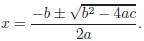
The quantity b2 − 4ac is sometimes called the discriminant of f, and written
disc(f).
Suppose f(x) = x2 + 1. Then disc(f) = −4 < 0, so f has no real roots.
This example is not purely artificial. In fact, you might
have come across this scenario when searching for
eigenvalues of linear transformations.
Suppose T : R2 → R2 is the linear transformation which rotates the plane 90°counterclockwise about the
origin. The matrix for T with respect to the standard basis is
The characteristic polynomial of this matrix is
 By the
previous example, it follows that A
By the
previous example, it follows that Ahas no real eigenvalues.
If we restrict ourselves to the real numbers, we see that
not every polynomial has a root (and hence not every
linear transformation has an eigenvalue). This seems quite unfortunate,
especially since the quadratic formula
seems to suggest what the roots (or eigenvalues) “should” be. To remedy this
situation, we will enlarge our
collection of numbers to include some of these “imaginary” roots. We’ll start by
simply adding

Definition. Let i represent a “number” which satisfies i2 = −1. We call
i the imaginary unit.
We’ll now add i to our collection of numbers.
Definition. We define the complex numbers to be the
set
C = {a + ib | a, b ∈ R}.
We define addition and multiplication of complex numbers
using the relation i2 = −1. That is, given complex
numbers a1 + ib1, a2 + ib2, we define
(a1 + ib1) + (a2 + ib2) := (a1 + a2) + i(b1 + b2)
and
(a1 + ib1)(a2 + ib2) := (a1a2 − b1b2) + i(a1b2 + a2b1).
(1) Suppose f(x) = x2 + 4. We claim the roots of f are x = ±2i. Indeed, observe that
f(±2i) = (±2i)2 + 4 = 4i2 + 4 = 4(−1) + 4 = 0.
Note that this agrees with the roots predicted by the quadratic formula:
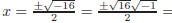
±2i.
(2) Suppose f(x) = x2+2x+3. Using the quadratic formula, the predicted roots of f are
 As a check, we compute
MatLab can natively work with complex numbers. For example, the above computation is entered
as follows:
>> (-1+sqrt(2)*i)^2+2*(-1+sqrt(2)*i)+3
ans =
-4.4409e-016
Notice that MatLab has introduced a small rounding error, outputting a result of −4.4409x10⁻¹⁶ ≈ 0.
Exercise 1. Use MatLab to compute (1 − 2i)5.
You might be worried we will need to keep adding new “numbers” to our collection
as we attempt to find
roots of polynomials of higher degrees. The following theorem, known as the
Fundamental Theorem of Algebra,
ensures we won’t need to extend our collection any further.
Theorem. Let p(x) = anxn + · · · + a1x + a0 be a polynomial, with ai ∈ C and an≠ 0. Then
p(x) = an(x − r1) · · · (x − rn)
for some r1, . . . , rn ∈ C.
In other words, when working with the complex numbers, every polynomial of
degree n has n (not necessarily
distinct) roots. This theorem may seem more amazing in light of the fact there
do not exist formulas for the
roots of general polynomials of degree five or more; that is, we can’t prove the
theorem by simply writing down
the roots of a general polynomial and checking they’re all in our set C.
The roots of x2 + 1 are x = ±i, which we can express as
x2 + 1 = (x − i)(x + i).
In general, finding the roots of a polynomial is quite difficult. Fortunately,
MatLab can do this for us. First
we must define our polynomial. MatLab stores polynomials as row vectors, with
components given by the
coefficients of the monomials. For example, to store the polynomial p(x) = x5 −
2x + 3, we enter
>> p=[1 0 0 0 -2 3];
To find the roots of p we use the roots command:
>> r=roots(p)
r =
-1.4236
-0.2467 + 1.3208i
-0.2467 - 1.3208i
0.9585 + 0.4984i
0.9585 - 0.4984i
As predicted by the previous theorem, the degree five polynomial p has five complex roots.
Exercise 2. Use MatLab to find the roots of the polynomial p(x) = x4 − 2x3 + 1.
Since we’ll be working with the complex numbers, it will be useful to have a few
additional definitions.
Definition. Suppose z ∈ C is given by z = a + ib, with a, b ∈ R. We make the following definitions:
(1) The real number a is called the real part of z, and is denoted Re(z). A
complex number z with Re(z) = 0
is called purely imaginary.
(2) The real number b is called the imaginary part of z, and is denoted Im(z). A
complex number z with
Im(z) = 0 is called purely real.
(3) The complex conjugate of z, denoted by
 is given by
 = a − ib = Re(z) − iIm(z).
>> conj(-1+2*i)
ans =
-1.0000 - 2.0000i
Exercise 3. Prove that Re(z) =
 and Im(z) =

By the above exercise, any equation involving the real and imaginary parts of z
can be written in terms of z
and  This observation will be useful to remember when we discuss complex
functions in Section 2.
This observation will be useful to remember when we discuss complex
functions in Section 2.
It is often helpful to picture the complex numbers as lying in the plane, with
the real part along the horizontal
axis and the imaginary part along the vertical axis.
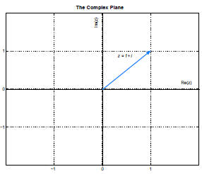
Unsurprisingly, this plane is called the complex plane. It was first described
by Caspar Wessel in 1799,
although it is also sometimes referred to as the Argand plane and credited to
Jean-Robert Argand. Use of
the complex plane was later popularized by Carl Gauss, and it was only after
this geometric interpretation
was introduced that the complex numbers became widely accepted. The complex
plane can be used to give
polar coordinates for z, with which one can deduce many beautiful relations.
Unfortunately, this would take us
beyond the scope of the current assignment.